
はじめに
離散時間信号をサンプリング周期に従ってDACから出力したときの周波数スペクトラムを計算する。量子化誤差は無視する。本記事の内容は下記の資料にも記した。
Release v0.8.0 · motchy869/Signal-Processing-Memorandum (github.com) 「0次ホールドされた離散時間信号の周波数スペクトラム」
\[
% to cope with definition mismatch between MathJax and LaTeX
\newcommand{\coloneq}{\mathrel{:=}}
\newcommand{\eqcolon}{\mathrel{=:}}
% general purpose
\newcommand{\ctext}[1]{\raise0.2ex\hbox{\textcircled{\scriptsize{#1}}}}
% mathematics
% general purpose
\DeclarePairedDelimiterX{\parens}[1]{\lparen}{\rparen}{#1}
\DeclarePairedDelimiterX{\braces}[1]{\lbrace}{\rbrace}{#1}
\DeclarePairedDelimiterX{\bracks}[1]{\lbrack}{\rbrack}{#1}
\DeclarePairedDelimiterX{\verts}[1]{|}{|}{#1}
\DeclarePairedDelimiterX{\Verts}[1]{\|}{\|}{#1}
\DeclarePairedDelimiterX{\setComprehension}[2]{\lbrace}{\rbrace}{#1\,\delimsize\vert\,#2}
\newcommand{\as}{{\quad\textrm{as}\quad}}
\newcommand{\st}{{\textrm{ s.t. }}}
\newcommand{\naturalNumbers}{\mathbb{N}}
\newcommand{\integers}{\mathbb{Z}}
\newcommand{\rationalNumbers}{\mathbb{Q}}
\newcommand{\realNumbers}{\mathbb{R}}
\newcommand{\nonNegRealNumbers}{\mathbb{R}_{\geq 0}}
\newcommand{\posRealNumbers}{\mathbb{R}_{> 0}}
\newcommand{\complexNumbers}{\mathbb{C}}
\newcommand{\field}{\mathbb{F}}
\newcommand{\EuclideanSpace}{\mathbb{E}}
\newcommand{\argmax}{\operatorname*{arg~max}}
\newcommand{\argmin}{\operatorname*{arg~min}}
% set theory
\newcommand{\range}[2]{\braces*{#1,\dotsc,#2}}
\renewcommand{\complement}{\mathrm{c}}
\newcommand{\ind}[2]{\mathbbm{1}_{#1}\parens*{#2}}
\newcommand{\indII}[1]{\mathbbm{1}\braces*{#1}}
% number theory
\newcommand{\abs}[1]{\verts*{#1}}
\newcommand{\combi}[2]{{_{#1}\mathrm{C}_{#2}}}
\newcommand{\perm}[2]{{_{#1}\mathrm{P}_{#2}}}
\newcommand{\GaloisField}{\mathrm{GF}}
% real analysis
\newcommand{\NapierE}{\mathrm{e}}
\newcommand{\sgn}{\operatorname{sgn}} % sign function
\newcommand{\rect}{\operatorname{rect}} % rectangular function
\newcommand{\cl}{\operatorname{cl}} % closure of a set
\newcommand{\img}{\operatorname{im}} % image of a function
\newcommand{\dom}{\operatorname{dom}} % domain of a function
\newcommand{\LittleO}[2]{\underset{#1}{o}\parens*{#2}} % little-o notation
\newcommand{\norm}[1]{\Verts*{#1}} % norm of a vector or function
\newcommand{\floor}[1]{\left\lfloor #1\right\rfloor}
\newcommand{\ceil}[1]{\left\lceil#1\right\rceil}
\newcommand{\sinc}{\operatorname{sinc}}
\newcommand{\nrmSinc}{\operatorname{nsinc}} % normalized sinc function
\newcommand{\erf}{\operatorname{erf}}
% inverse trigonometric functions
\newcommand{\asin}{\operatorname{Sin}^{-1}}
\newcommand{\acos}{\operatorname{Cos}^{-1}}
\newcommand{\atan}{\operatorname{Tan}^{-1}}
% derivative
\newcommand{\deriv}[3]{\frac{\mathrm{d}^{#3}#1}{\mathrm{d}{#2}^{#3}}}
\newcommand{\derivLong}[3]{\frac{\mathrm{d}^{#3}}{\mathrm{d}{#2}^{#3}}#1}
\newcommand{\partDeriv}[3]{\frac{\mathrm{\partial}^{#3}#1}{\mathrm{\partial}{#2}^{#3}}}
\newcommand{\partDerivLong}[3]{\frac{\mathrm{\partial}^{#3}}{\mathrm{\partial}{#2}^{#3}}#1}
\newcommand{\partDerivIIHetero}[3]{\frac{\mathrm{\partial}^2#1}{\partial#2\mathrm{\partial}#3}}
\newcommand{\partDerivIIHeteroLong}[3]{{\frac{\mathrm{\partial}^2}{\partial#2\mathrm{\partial}#3}#1}}
% integral
\newcommand{\pv}{{\textrm{ p.v. }}}
\newcommand{\integrate}[5]{\int_{#1}^{#2}{#3}{\;\mathrm{d}^{#4}}#5}
\newcommand{\LebInteg}[4]{\int_{#1} {#2} {#3}\parens*{\;\mathrm{d}#4}}
% complex analysis
\newcommand{\conj}[1]{\overline{#1}}
\renewcommand{\Re}{\operatorname{Re}}
\renewcommand{\Im}{\operatorname{Im}}
\newcommand{\Arg}{\operatorname{Arg}}
\newcommand{\Log}{\operatorname{Log}}
% Laplace transform
\newcommand{\LPLC}{\operatorname{\mathcal{L}}}
\newcommand{\ILPLC}{\operatorname{\mathcal{L}}^{-1}}
% discrete fourier transform
\newcommand{\DFT}{\operatorname{DFT}}
\newcommand{\IDFT}{\operatorname{IDFT}}
% Z-transform
\newcommand{\ZTrans}{\operatorname{\mathcal{Z}}}
\newcommand{\IZTrans}{\operatorname{\mathcal{Z}}^{-1}}
\newcommand{\SSZTrans}{\underset{\text{s.s.}}{\mathcal{Z}}} % single-sided Z-transform
% linear algebra
\newcommand{\bm}[1]{{\boldsymbol{#1}}}
\newcommand{\vecEntry}[2]{\bm{#1}\bracks*{#2}}
\newcommand{\matEntry}[3]{#1\bracks*{#2}\bracks*{#3}}
\newcommand{\matPart}[5]{\matEntry{#1}{#2:#3}{#4:#5}}
\newcommand{\minor}[3]{{#1}\bracks*{\setminus #2}\bracks*{\setminus #3}} % the minor of a matrix: row #2 and column #3 deleted
\newcommand{\diag}{\operatorname{diag}}
\newcommand{\transpose}[1]{{#1}^\top}
\newcommand{\HerConj}[1]{{#1}^*}
\newcommand{\tr}{\operatorname{tr}}
\newcommand{\inProd}[2]{\left\langle#1,#2\right\rangle}
\newcommand{\dotProd}[2]{#1 \cdot #2}
\newcommand{\HadamardProd}{\odot}
\newcommand{\HadamardDiv}{\oslash}
\newcommand{\vecSpan}{\operatorname{span}}
\newcommand{\rank}{\operatorname{rank}}
% vector
% unit vector
\newcommand{\vix}{\bm{i}_x}
\newcommand{\viy}{\bm{i}_y}
\newcommand{\viz}{\bm{i}_z}
% graph theory
\newcommand{\neighborhood}{\mathcal{N}}
% probability theory
\newcommand{\PDF}{\operatorname{PDF}}
\newcommand{\Ber}{\operatorname{Ber}}
\newcommand{\Beta}{\operatorname{Beta}}
\newcommand{\ExpDist}{\operatorname{ExpDist}}
\newcommand{\ErlangDist}{\operatorname{ErlangDist}}
\newcommand{\PoissonDist}{\operatorname{PoissonDist}}
\newcommand{\GammaDist}{\operatorname{Gamma}}
\newcommand{\cind}[2]{\ind{#1\left| #2\right.}} % conditional indicator function
\renewcommand{\Pr}{\operatorname{Pr}}
\DeclarePairedDelimiterX{\cPrParens}[2]{(}{)}{#1\,\delimsize\vert\,#2}
\newcommand{\Ev}{\operatorname{E}} % expected value
\newcommand{\Var}{\operatorname{Var}}
\newcommand{\Cov}{\operatorname{Cov}}
% physics
% unit of measurement
\newcommand{\second}{\text{s}}
\newcommand{\hertz}{\text{Hz}}
\newcommand{\decibel}{\text{dB}}
% signal processing
% Discrete Time Fourier Transform
\newcommand{\DTFT}{\operatorname{DTFT}}
\newcommand{\IDTFT}{\operatorname{IDTFT}}
% computer science
% fixed-point arithmetic
\newcommand{\IntPartBW}[1]{\underbracket[0.140ex]{#1}_\mathrm{i}} % 0.140ex is half of the default thickness. See: [How to make underbracket thinner](https://tex.stackexchange.com/questions/559078/how-to-make-underbracket-thinner)
\newcommand{\DecPartBW}[1]{\underbracket[0.140ex]{#1}_\mathrm{d}}
\newcommand{\TotalBW}[1]{\underbracket[0.140ex]{#1}}
\newcommand{\Rat}{\operatorname{Rat}} % Maps a fixed-point number to a corresponding rational number.
% programming
\newcommand{\plpl}{\mathrel{++}}
\newcommand{\pleq}{\mathrel{+}=}
\newcommand{\asteq}{\mathrel{*}=}
\]
主張
\[
\newcommand{\xd}{x_\text{d}}
\newcommand{\Xd}{X_\text{d}}
\newcommand{\Ts}{T_\text{s}}
\newcommand{\FT}{\mathcal{F}}
\]
$\xd:\integers\to\complexNumbers$ を離散時間信号とする。$\Xd$ を $\xd$ のDTFTとする。$\Ts>0$ をサンプル周期として $\xd$ の0次ホールドで生成した階段状の連続時間信号を $x$ とする。
$u:\realNumbers\to\braces{0,1}$ を幅 $\Ts$ のパルスとする。
\[ u(t) = \begin{cases} 1 & 0\leq t < \Ts \\ 0 & \text{otherwise} \end{cases} \]$x$ は次式で表される。
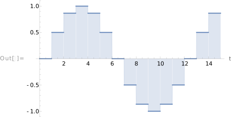
\[ x(t) = \sum_{n=-\infty}^\infty \xd(n)u(t-n\Ts) \]次の図は $\Ts=1,\xd(n) = \sin\parens{2\pi n/12}\;(0\leq n\leq 24),\;\xd(n) = 0\;(n<0,24<n)$ の例である。
$x$ のFourier変換 $X$ は次式である。
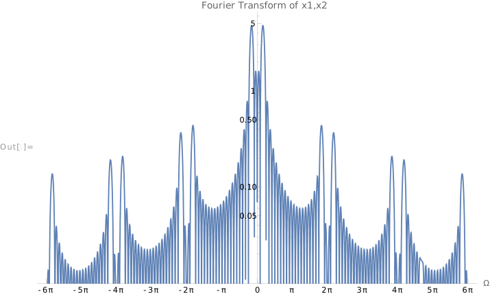
\[ X(\omega) = \frac{\Ts}{\sqrt{2\pi}}\exp\parens*{-i\frac{\Ts}{2}\omega}\parens*{\sinc \frac{\Ts}{2}\omega}\Xd(\omega) \]$\Xd(\omega)$ が $2\pi/\Ts$ 周期関数であることに注意すれば、$\Xd(\omega)$ の第1 Nyquist領域の形状が位相回転 $\exp\parens{-i \omega\Ts/2}$ とレベル減衰 $\sinc\omega\Ts/2$ を伴いつつ周期的に無限に繰り返されていることがわかる。この現象は「アパーチャ効果」と呼ばれる。
次の図は図1に対応する $X$ の例である。
導出
\[ X(\omega) = \FT\parens*{\sum_{n=-\infty}^\infty \xd(n)u(t-n\Ts)}(\omega) = \sum_{n=-\infty}^\infty \xd(n)\FT\parens*{u(t-n\Ts)}(\omega) \tag{1} \]ここで次式が成り立つ。
\begin{align*} \FT\parens*{u(t-n\Ts)}(\omega) &= \exp\parens*{-i \omega n\Ts}\FT\parens*{u}(\omega) = \exp\parens*{-i \omega n\Ts}\frac{1}{\sqrt{2\pi}}\integrate{0}{\Ts}{\exp\parens*{-i\omega t}}{}{t} \\ &= \frac{i}{\omega\sqrt{2\pi}}\parens*{\exp\parens*{-i \omega\Ts}-1}\exp\parens*{-i \omega n\Ts} \\ &= \frac{i}{\omega\sqrt{2\pi}}\exp\parens{-i \omega n\Ts}\exp\parens{-i \omega\Ts/2}\parens*{\exp\parens*{-i \omega\Ts/2} – \exp\parens*{i \omega\Ts/2}} \\ &= \frac{i}{\omega\sqrt{2\pi}}\exp\parens{-i \omega n\Ts}\exp\parens{-i \omega\Ts/2}(-2i)\sin\frac{\omega\Ts}{2} \\ &= \frac{2}{\omega\sqrt{2\pi}}\exp\parens{-i \omega n\Ts}\exp\parens{-i \omega\Ts/2}\sin\frac{\omega\Ts}{2} \\ &= \frac{\Ts}{\sqrt{2\pi}}\exp\parens{-i \omega n\Ts}\exp\parens{-i \omega\Ts/2}\sinc\frac{\omega\Ts}{2} \end{align*}これを式(1)に適用して次式を得る。
\begin{align*} X(\omega) &= \sum_{n=-\infty}^\infty \xd(n)\frac{\Ts}{\sqrt{2\pi}}\exp\parens{-i \omega n\Ts}\exp\parens{-i \omega\Ts/2}\sinc\frac{\omega\Ts}{2} \\ &= \frac{\Ts}{\sqrt{2\pi}}\exp\parens{-i \omega\Ts/2}\sinc\frac{\omega\Ts}{2} \sum_{n=-\infty}^\infty \xd(n)\exp\parens{-i \omega n\Ts} \\ &= \frac{\Ts}{\sqrt{2\pi}}\exp\parens*{-i\frac{\Ts}{2}\omega}\parens*{\sinc \frac{\Ts}{2}\omega}\Xd(\omega) \end{align*}$\square$
コメントを残す
コメントを投稿するにはログインしてください。