はじめに
離散時間信号を DA 変換した結果の Fourier 変換には sinc 関数状のゲイン歪みが積の形で含まれる。本記事では DA 変換の直前に、上手く設計された10タップ程度の FIR フィルタを掛けてこの影響を緩和する方法を述べる。
本記事の内容は下記の資料にも記した。
Release v0.11.1 · motchy869/Signal-Processing-Memorandum (github.com) 「inverse-sinc-filter」
\[
% to cope with definition mismatch between MathJax and LaTeX
\newcommand{\coloneq}{\mathrel{:=}}
\newcommand{\eqcolon}{\mathrel{=:}}
% general purpose
\newcommand{\ctext}[1]{\raise0.2ex\hbox{\textcircled{\scriptsize{#1}}}}
% mathematics
% general purpose
\DeclarePairedDelimiterX{\parens}[1]{\lparen}{\rparen}{#1}
\DeclarePairedDelimiterX{\braces}[1]{\lbrace}{\rbrace}{#1}
\DeclarePairedDelimiterX{\bracks}[1]{\lbrack}{\rbrack}{#1}
\DeclarePairedDelimiterX{\verts}[1]{|}{|}{#1}
\DeclarePairedDelimiterX{\Verts}[1]{\|}{\|}{#1}
\DeclarePairedDelimiterX{\setComprehension}[2]{\lbrace}{\rbrace}{#1\,\delimsize\vert\,#2}
\newcommand{\as}{{\quad\textrm{as}\quad}}
\newcommand{\st}{{\textrm{ s.t. }}}
\newcommand{\naturalNumbers}{\mathbb{N}}
\newcommand{\integers}{\mathbb{Z}}
\newcommand{\rationalNumbers}{\mathbb{Q}}
\newcommand{\realNumbers}{\mathbb{R}}
\newcommand{\nonNegRealNumbers}{\mathbb{R}_{\geq 0}}
\newcommand{\posRealNumbers}{\mathbb{R}_{> 0}}
\newcommand{\complexNumbers}{\mathbb{C}}
\newcommand{\field}{\mathbb{F}}
\newcommand{\EuclideanSpace}{\mathbb{E}}
\newcommand{\argmax}{\operatorname*{arg~max}}
\newcommand{\argmin}{\operatorname*{arg~min}}
% set theory
\newcommand{\range}[2]{\braces*{#1,\dotsc,#2}}
\renewcommand{\complement}{\mathrm{c}}
\newcommand{\ind}[2]{\mathbbm{1}_{#1}\parens*{#2}}
\newcommand{\indII}[1]{\mathbbm{1}\braces*{#1}}
% number theory
\newcommand{\abs}[1]{\verts*{#1}}
\newcommand{\combi}[2]{{_{#1}\mathrm{C}_{#2}}}
\newcommand{\perm}[2]{{_{#1}\mathrm{P}_{#2}}}
\newcommand{\GaloisField}{\mathrm{GF}}
% real analysis
\newcommand{\NapierE}{\mathrm{e}}
\newcommand{\sgn}{\operatorname{sgn}} % sign function
\newcommand{\rect}{\operatorname{rect}} % rectangular function
\newcommand{\cl}{\operatorname{cl}} % closure of a set
\newcommand{\img}{\operatorname{im}} % image of a function
\newcommand{\dom}{\operatorname{dom}} % domain of a function
\newcommand{\LittleO}[2]{\underset{#1}{o}\parens*{#2}} % little-o notation
\newcommand{\norm}[1]{\Verts*{#1}} % norm of a vector or function
\newcommand{\floor}[1]{\left\lfloor #1\right\rfloor}
\newcommand{\ceil}[1]{\left\lceil#1\right\rceil}
\newcommand{\sinc}{\operatorname{sinc}}
\newcommand{\nrmSinc}{\operatorname{nsinc}} % normalized sinc function
\newcommand{\erf}{\operatorname{erf}}
% inverse trigonometric functions
\newcommand{\asin}{\operatorname{Sin}^{-1}}
\newcommand{\acos}{\operatorname{Cos}^{-1}}
\newcommand{\atan}{\operatorname{Tan}^{-1}}
% derivative
\newcommand{\deriv}[3]{\frac{\mathrm{d}^{#3}#1}{\mathrm{d}{#2}^{#3}}}
\newcommand{\derivLong}[3]{\frac{\mathrm{d}^{#3}}{\mathrm{d}{#2}^{#3}}#1}
\newcommand{\partDeriv}[3]{\frac{\mathrm{\partial}^{#3}#1}{\mathrm{\partial}{#2}^{#3}}}
\newcommand{\partDerivLong}[3]{\frac{\mathrm{\partial}^{#3}}{\mathrm{\partial}{#2}^{#3}}#1}
\newcommand{\partDerivIIHetero}[3]{\frac{\mathrm{\partial}^2#1}{\partial#2\mathrm{\partial}#3}}
\newcommand{\partDerivIIHeteroLong}[3]{{\frac{\mathrm{\partial}^2}{\partial#2\mathrm{\partial}#3}#1}}
% integral
\newcommand{\pv}{{\textrm{ p.v. }}}
\newcommand{\integrate}[5]{\int_{#1}^{#2}{#3}{\;\mathrm{d}^{#4}}#5}
\newcommand{\LebInteg}[4]{\int_{#1} {#2} {#3}\parens*{\;\mathrm{d}#4}}
% complex analysis
\newcommand{\conj}[1]{\overline{#1}}
\renewcommand{\Re}{\operatorname{Re}}
\renewcommand{\Im}{\operatorname{Im}}
\newcommand{\Arg}{\operatorname{Arg}}
\newcommand{\Log}{\operatorname{Log}}
% Laplace transform
\newcommand{\LPLC}{\operatorname{\mathcal{L}}}
\newcommand{\ILPLC}{\operatorname{\mathcal{L}}^{-1}}
% discrete fourier transform
\newcommand{\DFT}{\operatorname{DFT}}
\newcommand{\IDFT}{\operatorname{IDFT}}
% Z-transform
\newcommand{\ZTrans}{\operatorname{\mathcal{Z}}}
\newcommand{\IZTrans}{\operatorname{\mathcal{Z}}^{-1}}
\newcommand{\SSZTrans}{\underset{\text{s.s.}}{\mathcal{Z}}} % single-sided Z-transform
% linear algebra
\newcommand{\bm}[1]{{\boldsymbol{#1}}}
\newcommand{\vecEntry}[2]{\bm{#1}\bracks*{#2}}
\newcommand{\matEntry}[3]{#1\bracks*{#2}\bracks*{#3}}
\newcommand{\matPart}[5]{\matEntry{#1}{#2:#3}{#4:#5}}
\newcommand{\minor}[3]{{#1}\bracks*{\setminus #2}\bracks*{\setminus #3}} % the minor of a matrix: row #2 and column #3 deleted
\newcommand{\diag}{\operatorname{diag}}
\newcommand{\transpose}[1]{{#1}^\top}
\newcommand{\HerConj}[1]{{#1}^*}
\newcommand{\tr}{\operatorname{tr}}
\newcommand{\inProd}[2]{\left\langle#1,#2\right\rangle}
\newcommand{\dotProd}[2]{#1 \cdot #2}
\newcommand{\HadamardProd}{\odot}
\newcommand{\HadamardDiv}{\oslash}
\newcommand{\vecSpan}{\operatorname{span}}
\newcommand{\rank}{\operatorname{rank}}
% vector
% unit vector
\newcommand{\vix}{\bm{i}_x}
\newcommand{\viy}{\bm{i}_y}
\newcommand{\viz}{\bm{i}_z}
% graph theory
\newcommand{\neighborhood}{\mathcal{N}}
% probability theory
\newcommand{\PDF}{\operatorname{PDF}}
\newcommand{\Ber}{\operatorname{Ber}}
\newcommand{\Beta}{\operatorname{Beta}}
\newcommand{\ExpDist}{\operatorname{ExpDist}}
\newcommand{\ErlangDist}{\operatorname{ErlangDist}}
\newcommand{\PoissonDist}{\operatorname{PoissonDist}}
\newcommand{\GammaDist}{\operatorname{Gamma}}
\newcommand{\cind}[2]{\ind{#1\left| #2\right.}} % conditional indicator function
\renewcommand{\Pr}{\operatorname{Pr}}
\DeclarePairedDelimiterX{\cPrParens}[2]{(}{)}{#1\,\delimsize\vert\,#2}
\newcommand{\Ev}{\operatorname{E}} % expected value
\newcommand{\Var}{\operatorname{Var}}
\newcommand{\Cov}{\operatorname{Cov}}
% physics
% unit of measurement
\newcommand{\second}{\text{s}}
\newcommand{\hertz}{\text{Hz}}
\newcommand{\decibel}{\text{dB}}
% signal processing
% Discrete Time Fourier Transform
\newcommand{\DTFT}{\operatorname{DTFT}}
\newcommand{\IDTFT}{\operatorname{IDTFT}}
% computer science
% fixed-point arithmetic
\newcommand{\IntPartBW}[1]{\underbracket[0.140ex]{#1}_\mathrm{i}} % 0.140ex is half of the default thickness. See: [How to make underbracket thinner](https://tex.stackexchange.com/questions/559078/how-to-make-underbracket-thinner)
\newcommand{\DecPartBW}[1]{\underbracket[0.140ex]{#1}_\mathrm{d}}
\newcommand{\TotalBW}[1]{\underbracket[0.140ex]{#1}}
\newcommand{\Rat}{\operatorname{Rat}} % Maps a fixed-point number to a corresponding rational number.
% programming
\newcommand{\plpl}{\mathrel{++}}
\newcommand{\pleq}{\mathrel{+}=}
\newcommand{\asteq}{\mathrel{*}=}
\]
\[
\newcommand{\Ts}{T_\text{s}}
\]
背景
離散時間信号を量子化誤差なく完璧にDA変換した結果のFourier変換には次式で表される変化が積の形で含まれることを以前の記事「理想的なDACの出力の周波数スペクトラム」で述べた。
\[ \sinc \frac{\Ts}{2}\omega = \sinc \frac{\Omega}{2} \]
ここに $\Ts$ はサンプリング周期, $\Omega$ は正規化各周波数である。変化の中には上式の他に $\exp\parens*{-i\frac{\Ts}{2}\omega}$ という項も含まれるが、これは一定の群遅延が加わる(線形位相特性)だけであり、実用上無害なので無視する。次の図は $\abs{\sinc \frac{\Omega}{2}}$ をプロットしたものである。
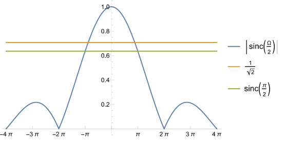 図1 量子化誤差のないDA変換結果の sinc 状ゲイン歪み
上の図から、第1 Nyquist 領域の端 $-\pi, \pi$ で約 -3dB のゲイン低下が生じていることが解る。実は0次ホールドで出力する直前に、上手く設計された10タップ程度の FIR フィルタを掛けてこの影響を緩和し、下図のようなゲイン特性に変更できる。このフィルタは一般に 「inverse-sinc フィルタ」と呼ばれる。
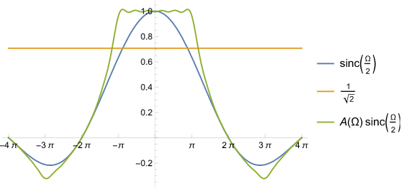 図2 inverse-sinc フィルタによって緩和されたゲイン歪み
inverse-sinc filter は $[-\pi, \pi]$ で sinc 状歪みの逆特性を近似するフィルタである。DA変換の対象とする信号は通常、サンプリング定理を念頭に置いてスペクトラムが $[-\pi,\pi]$ の領域に収まる信号であるから、上述の補正が十分に機能する。以下ではこのフィルタの設計方法の1つを述べる。
係数の導出
大雑把に言えば、フィルタ係数に対応する DTFT が $[-\pi,\pi]$ で $1/\sinc(\Omega/2)$ を近似するように最小二乗法で係数を決定する。
フィルタ係数 $a:\integers\to\realNumbers$ は偶対称な実数値関数とし、非零の係数の個数を奇数とする。数式で述べれば $N\in\naturalNumbers,\;\forall n\in\integers\;a(-n) = a(n),\forall n>N,\;\;a(n) = 0$ である。この制約条件が唯一の方法ではないだろうが、後に見るようにこれで十分な性能を得られる。
$a$ の DTFT を $A$ とする。すなわち
\[ A(\Omega) = \sum_{n=-N}^N a(n)\exp(-i\Omega n) = a(0) + 2\sum_{n=1}^N a(n)\cos(\Omega n) = \bm{v}(\Omega)^\top\bm{a} \]
ここに $\bm{v}(\Omega) \coloneqq [1, 2\cos\Omega,\dots,2\cos N\Omega]^\top\in\realNumbers^{N+1},\;\bm{a} = [a(0),\dots,a(N)]^\top\in\realNumbers^{N+1}$ である。$[-\pi,\pi]$ で $A$ が $1/\sinc(\Omega/2)$ を近似するように次式を最小化する $a$ を求める。
\[ \integrate{-\pi}{\pi}{\norm{A(\Omega) – 1/\sinc(\Omega/2)}_2^2}{}{\Omega} \tag{1} \]
被積分関数の中身を展開すると次式を得る。
\[ \norm{A(\Omega) – 1/\sinc(\Omega/2)}_2^2 = \bm{a}^\top\bm{v}(\Omega)\bm{v}(\Omega)^\top\bm{a} – \frac{2}{\sinc(\Omega/2)}\bm{v}(\Omega)^\top\bm{a} + 1/\sinc(\Omega/2)^2 \]
これを式(1)に適用すると次式を得る。
\[ (1) = \bm{a}^\top M\bm{a} – 2\bm{m}^\top\bm{a} + \integrate{-\pi}{\pi}{1/\sinc(\Omega/2)^2}{}{\Omega} \tag{2} \]
ここに $M,\bm{m}$ は次式で定義される数である。
\[ M \coloneqq \integrate{-\pi}{\pi}{\bm{v}(\Omega)\bm{v}(\Omega)^\top}{}{\Omega} = 2\pi\diag\parens*{1,2,2,\dots,2},\quad \bm{m} = \integrate{-\pi}{\pi}{\bm{v}(\Omega)^\top/\sinc(\Omega/2)}{}{\Omega} \]
$\bm{m}$ は数値計算で求める。式(2)の中で $\bm{a}$ に依存しない項を無視すると、最小化すべき関数は次式である。
\[ f_\text{cost}(\bm{a}) = \bm{a}^\top M\bm{a} – 2\bm{m}^\top\bm{a} \]
これは狭義凸関数であり $(\nabla f_\text{cost})(\bm{a}) = 2(M\bm{a} – \bm{m})$ なので $f$ を最小化する $\bm{a}$ を $\bm{a}_\text{opt}$ とするとこれは $M^{-1}\bm{m} = \diag\parens*{m_0,m_1 /2,\dots,m_N /2}/(2\pi)$ である。ここに $m_i\;(i=0,1,\dots,N)$ は $\bm{m}$ の第 $i$ 要素である。
数値例
$N=5$ のとき $\bm{a}_\text{opt} \approx [1.166240, -0.106996, 0.034475, -0.016454, 0.009530, -0.006189]^\top$ を得る。次の図はこの係数をプロットしたものである。
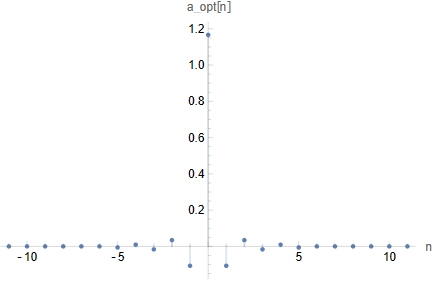 図3 inverse-sinc フィルタの係数(N=5)
次の図は、この係数に対応するフィルタのインパルス応答の DTFT と $1/\sinc(\Omega/2)$ を比較したものである。
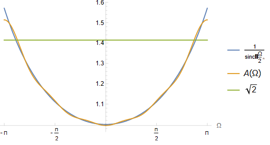 図4 inverse-sinc フィルタのインパルス応答の DTFT
このフィルタを使ってゲイン歪みを緩和したのが先に挙げた図2である。

コメントを残す
コメントを投稿するにはログインしてください。