\[
% to cope with definition mismatch between MathJax and LaTeX
\newcommand{\coloneq}{\mathrel{:=}}
\newcommand{\eqcolon}{\mathrel{=:}}
% general purpose
\newcommand{\ctext}[1]{\raise0.2ex\hbox{\textcircled{\scriptsize{#1}}}}
% mathematics
% general purpose
\DeclarePairedDelimiterX{\parens}[1]{\lparen}{\rparen}{#1}
\DeclarePairedDelimiterX{\braces}[1]{\lbrace}{\rbrace}{#1}
\DeclarePairedDelimiterX{\bracks}[1]{\lbrack}{\rbrack}{#1}
\DeclarePairedDelimiterX{\verts}[1]{|}{|}{#1}
\DeclarePairedDelimiterX{\Verts}[1]{\|}{\|}{#1}
\DeclarePairedDelimiterX{\setComprehension}[2]{\lbrace}{\rbrace}{#1\,\delimsize\vert\,#2}
\newcommand{\as}{{\quad\textrm{as}\quad}}
\newcommand{\st}{{\textrm{ s.t. }}}
\newcommand{\naturalNumbers}{\mathbb{N}}
\newcommand{\integers}{\mathbb{Z}}
\newcommand{\rationalNumbers}{\mathbb{Q}}
\newcommand{\realNumbers}{\mathbb{R}}
\newcommand{\nonNegRealNumbers}{\mathbb{R}_{\geq 0}}
\newcommand{\posRealNumbers}{\mathbb{R}_{> 0}}
\newcommand{\complexNumbers}{\mathbb{C}}
\newcommand{\field}{\mathbb{F}}
\newcommand{\EuclideanSpace}{\mathbb{E}}
\newcommand{\argmax}{\operatorname*{arg~max}}
\newcommand{\argmin}{\operatorname*{arg~min}}
% set theory
\newcommand{\range}[2]{\braces*{#1,\dotsc,#2}}
\renewcommand{\complement}{\mathrm{c}}
\newcommand{\ind}[2]{\mathbbm{1}_{#1}\parens*{#2}}
\newcommand{\indII}[1]{\mathbbm{1}\braces*{#1}}
% number theory
\newcommand{\abs}[1]{\verts*{#1}}
\newcommand{\combi}[2]{{_{#1}\mathrm{C}_{#2}}}
\newcommand{\perm}[2]{{_{#1}\mathrm{P}_{#2}}}
\newcommand{\GaloisField}{\mathrm{GF}}
% real analysis
\newcommand{\NapierE}{\mathrm{e}}
\newcommand{\sgn}{\operatorname{sgn}} % sign function
\newcommand{\rect}{\operatorname{rect}} % rectangular function
\newcommand{\cl}{\operatorname{cl}} % closure of a set
\newcommand{\img}{\operatorname{im}} % image of a function
\newcommand{\dom}{\operatorname{dom}} % domain of a function
\newcommand{\LittleO}[2]{\underset{#1}{o}\parens*{#2}} % little-o notation
\newcommand{\norm}[1]{\Verts*{#1}} % norm of a vector or function
\newcommand{\floor}[1]{\left\lfloor #1\right\rfloor}
\newcommand{\ceil}[1]{\left\lceil#1\right\rceil}
\newcommand{\sinc}{\operatorname{sinc}}
\newcommand{\nrmSinc}{\operatorname{nsinc}} % normalized sinc function
\newcommand{\erf}{\operatorname{erf}}
% inverse trigonometric functions
\newcommand{\asin}{\operatorname{Sin}^{-1}}
\newcommand{\acos}{\operatorname{Cos}^{-1}}
\newcommand{\atan}{\operatorname{Tan}^{-1}}
% derivative
\newcommand{\deriv}[3]{\frac{\mathrm{d}^{#3}#1}{\mathrm{d}{#2}^{#3}}}
\newcommand{\derivLong}[3]{\frac{\mathrm{d}^{#3}}{\mathrm{d}{#2}^{#3}}#1}
\newcommand{\partDeriv}[3]{\frac{\mathrm{\partial}^{#3}#1}{\mathrm{\partial}{#2}^{#3}}}
\newcommand{\partDerivLong}[3]{\frac{\mathrm{\partial}^{#3}}{\mathrm{\partial}{#2}^{#3}}#1}
\newcommand{\partDerivIIHetero}[3]{\frac{\mathrm{\partial}^2#1}{\partial#2\mathrm{\partial}#3}}
\newcommand{\partDerivIIHeteroLong}[3]{{\frac{\mathrm{\partial}^2}{\partial#2\mathrm{\partial}#3}#1}}
% integral
\newcommand{\pv}{{\textrm{ p.v. }}}
\newcommand{\integrate}[5]{\int_{#1}^{#2}{#3}{\;\mathrm{d}^{#4}}#5}
\newcommand{\LebInteg}[4]{\int_{#1} {#2} {#3}\parens*{\;\mathrm{d}#4}}
% complex analysis
\newcommand{\conj}[1]{\overline{#1}}
\renewcommand{\Re}{\operatorname{Re}}
\renewcommand{\Im}{\operatorname{Im}}
\newcommand{\Arg}{\operatorname{Arg}}
\newcommand{\Log}{\operatorname{Log}}
% Laplace transform
\newcommand{\LPLC}{\operatorname{\mathcal{L}}}
\newcommand{\ILPLC}{\operatorname{\mathcal{L}}^{-1}}
% discrete fourier transform
\newcommand{\DFT}{\operatorname{DFT}}
\newcommand{\IDFT}{\operatorname{IDFT}}
% Z-transform
\newcommand{\ZTrans}{\operatorname{\mathcal{Z}}}
\newcommand{\IZTrans}{\operatorname{\mathcal{Z}}^{-1}}
\newcommand{\SSZTrans}{\underset{\text{s.s.}}{\mathcal{Z}}} % single-sided Z-transform
% linear algebra
\newcommand{\bm}[1]{{\boldsymbol{#1}}}
\newcommand{\vecEntry}[2]{\bm{#1}\bracks*{#2}}
\newcommand{\matEntry}[3]{#1\bracks*{#2}\bracks*{#3}}
\newcommand{\matPart}[5]{\matEntry{#1}{#2:#3}{#4:#5}}
\newcommand{\minor}[3]{{#1}\bracks*{\setminus #2}\bracks*{\setminus #3}} % the minor of a matrix: row #2 and column #3 deleted
\newcommand{\diag}{\operatorname{diag}}
\newcommand{\transpose}[1]{{#1}^\top}
\newcommand{\HerConj}[1]{{#1}^*}
\newcommand{\tr}{\operatorname{tr}}
\newcommand{\inProd}[2]{\left\langle#1,#2\right\rangle}
\newcommand{\dotProd}[2]{#1 \cdot #2}
\newcommand{\HadamardProd}{\odot}
\newcommand{\HadamardDiv}{\oslash}
\newcommand{\vecSpan}{\operatorname{span}}
\newcommand{\rank}{\operatorname{rank}}
% vector
% unit vector
\newcommand{\vix}{\bm{i}_x}
\newcommand{\viy}{\bm{i}_y}
\newcommand{\viz}{\bm{i}_z}
% graph theory
\newcommand{\neighborhood}{\mathcal{N}}
% probability theory
\newcommand{\PDF}{\operatorname{PDF}}
\newcommand{\Ber}{\operatorname{Ber}}
\newcommand{\Beta}{\operatorname{Beta}}
\newcommand{\ExpDist}{\operatorname{ExpDist}}
\newcommand{\ErlangDist}{\operatorname{ErlangDist}}
\newcommand{\PoissonDist}{\operatorname{PoissonDist}}
\newcommand{\GammaDist}{\operatorname{Gamma}}
\newcommand{\cind}[2]{\ind{#1\left| #2\right.}} % conditional indicator function
\renewcommand{\Pr}{\operatorname{Pr}}
\DeclarePairedDelimiterX{\cPrParens}[2]{(}{)}{#1\,\delimsize\vert\,#2}
\newcommand{\Ev}{\operatorname{E}} % expected value
\newcommand{\Var}{\operatorname{Var}}
\newcommand{\Cov}{\operatorname{Cov}}
% physics
% unit of measurement
\newcommand{\second}{\text{s}}
\newcommand{\hertz}{\text{Hz}}
\newcommand{\decibel}{\text{dB}}
% signal processing
% Discrete Time Fourier Transform
\newcommand{\DTFT}{\operatorname{DTFT}}
\newcommand{\IDTFT}{\operatorname{IDTFT}}
% computer science
% fixed-point arithmetic
\newcommand{\IntPartBW}[1]{\underbracket[0.140ex]{#1}_\mathrm{i}} % 0.140ex is half of the default thickness. See: [How to make underbracket thinner](https://tex.stackexchange.com/questions/559078/how-to-make-underbracket-thinner)
\newcommand{\DecPartBW}[1]{\underbracket[0.140ex]{#1}_\mathrm{d}}
\newcommand{\TotalBW}[1]{\underbracket[0.140ex]{#1}}
\newcommand{\Rat}{\operatorname{Rat}} % Maps a fixed-point number to a corresponding rational number.
% programming
\newcommand{\plpl}{\mathrel{++}}
\newcommand{\pleq}{\mathrel{+}=}
\newcommand{\asteq}{\mathrel{*}=}
\]
はじめに
リアルタイム信号処理に於いて、移動平均を高速に計算し続けたいシーンはよくある。窓をずらしながらステップ毎に総和の計算を行うと、1ステップあたりの計算量が$O(N)$($N$は窓の幅)であるが、これを何とかして再帰的に計算できれば1ステップあたりの計算量を窓の幅に依存しないようにできる。信号の長さが有限で、かつそれほど長くなければ、尺取り法で実現できる。しかし信号が入力され続ける場合、計算誤差が蓄積してしまう。本記事では真の移動平均とは少しだけ異なる近似値を計算するかわりに、再帰的に計算する方法を述べる。
方法1
 方法1のブロック図
計算量を定数にするために再帰型フィルタで構成する。$N\in\mathbb{N},\;\alpha\in(0,1)$ とする。
計算誤差を無視した場合の理想的な移動平均フィルタは $\alpha=1$ に対応するが、計算誤差のある現実の計算機で $\alpha=1$ とすると、時間の経過とともにループ部分に誤差が際限なく蓄積する。それを防ぐために $\alpha$ を1に十分近く(例えば0.999)とり、ループ部分の開ループゲインの絶対値を1未満にすることで、刻一刻生じる誤差がそれぞれ0に収束するようにする。入力 $u(n)$ の分岐で $N$ ステップ遅延させた信号に乗じている $\alpha^N$ は、ループ部分に入ったパルスを $N$ ステップ後にちょうど消し去るためのスケーリングである。
方法1の限界
$N$ が大きくなる(数十程度)につれ、適切な $\alpha$ を作れなくなる。$\alpha^N$ が1に比べて無視できないほど小さくなってしまうからである。$N$ を1に近づけることで緩和されるが、計算誤差に対する安定性が劣化する。
方法2
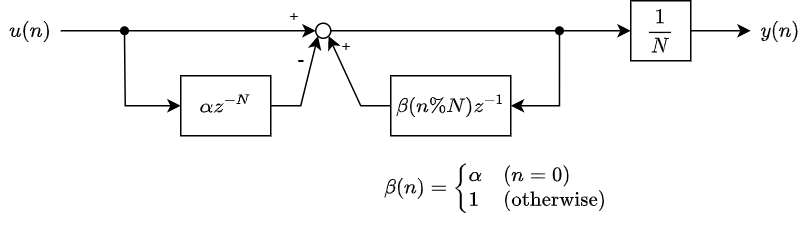 方法2のブロック図
方法1の欠点であった、大きい $N$ に対応できないという問題を克服する。ただし後述するがこのシステムは時不変ではない。
方法1で定義した記号は引き続き用いる。$\%$ は割り算の余りを表す。ループ部分は $N$ の倍数の時刻毎に開ループゲインが $\alpha$ となり、それ以外の時刻では1である。よって、任意の時刻にフィルタに入力されたパルスは、その $N$ ステップ遅延の $\alpha$ 倍がループ部分に逆符号で入るまでの間にループ部分でちょうど1回だけ $\alpha$ 倍されるため、両者が相殺する。刻一刻生じる計算誤差はループ部分で定期的に $\alpha$ 倍され縮小するため、フィルタが発散することはない。このフィルタのインパルス応答は時間に依存するため時不変ではないが、$\alpha$ が1に十分近ければ、理想応答との差は微々たるものである。

コメントを残す
コメントを投稿するにはログインしてください。