はじめに
今読んでいる本に、完全半波長ダイポールアンテナを直線上に配列したアレイアンテナが紹介されていた。配列軸と素子が平行な場合のbroadside型については放射指向性の数式が載っているが、配列軸と素子が垂直な場合のend-fire型は言及が浅く、数式が載っていないので導出してみた。broadside型,end-fire型両方について計算機による可視化もやってみた。
\[
% to cope with definition mismatch between MathJax and LaTeX
\newcommand{\coloneq}{\mathrel{:=}}
\newcommand{\eqcolon}{\mathrel{=:}}
% general purpose
\newcommand{\ctext}[1]{\raise0.2ex\hbox{\textcircled{\scriptsize{#1}}}}
% mathematics
% general purpose
\DeclarePairedDelimiterX{\parens}[1]{\lparen}{\rparen}{#1}
\DeclarePairedDelimiterX{\braces}[1]{\lbrace}{\rbrace}{#1}
\DeclarePairedDelimiterX{\bracks}[1]{\lbrack}{\rbrack}{#1}
\DeclarePairedDelimiterX{\verts}[1]{|}{|}{#1}
\DeclarePairedDelimiterX{\Verts}[1]{\|}{\|}{#1}
\DeclarePairedDelimiterX{\setComprehension}[2]{\lbrace}{\rbrace}{#1\,\delimsize\vert\,#2}
\newcommand{\as}{{\quad\textrm{as}\quad}}
\newcommand{\st}{{\textrm{ s.t. }}}
\newcommand{\naturalNumbers}{\mathbb{N}}
\newcommand{\integers}{\mathbb{Z}}
\newcommand{\rationalNumbers}{\mathbb{Q}}
\newcommand{\realNumbers}{\mathbb{R}}
\newcommand{\nonNegRealNumbers}{\mathbb{R}_{\geq 0}}
\newcommand{\posRealNumbers}{\mathbb{R}_{> 0}}
\newcommand{\complexNumbers}{\mathbb{C}}
\newcommand{\field}{\mathbb{F}}
\newcommand{\EuclideanSpace}{\mathbb{E}}
\newcommand{\argmax}{\operatorname*{arg~max}}
\newcommand{\argmin}{\operatorname*{arg~min}}
% set theory
\newcommand{\range}[2]{\braces*{#1,\dotsc,#2}}
\renewcommand{\complement}{\mathrm{c}}
\newcommand{\ind}[2]{\mathbbm{1}_{#1}\parens*{#2}}
\newcommand{\indII}[1]{\mathbbm{1}\braces*{#1}}
% number theory
\newcommand{\abs}[1]{\verts*{#1}}
\newcommand{\combi}[2]{{_{#1}\mathrm{C}_{#2}}}
\newcommand{\perm}[2]{{_{#1}\mathrm{P}_{#2}}}
\newcommand{\GaloisField}{\mathrm{GF}}
% real analysis
\newcommand{\NapierE}{\mathrm{e}}
\newcommand{\sgn}{\operatorname{sgn}} % sign function
\newcommand{\rect}{\operatorname{rect}} % rectangular function
\newcommand{\cl}{\operatorname{cl}} % closure of a set
\newcommand{\img}{\operatorname{im}} % image of a function
\newcommand{\dom}{\operatorname{dom}} % domain of a function
\newcommand{\LittleO}[2]{\underset{#1}{o}\parens*{#2}} % little-o notation
\newcommand{\norm}[1]{\Verts*{#1}} % norm of a vector or function
\newcommand{\floor}[1]{\left\lfloor #1\right\rfloor}
\newcommand{\ceil}[1]{\left\lceil#1\right\rceil}
\newcommand{\sinc}{\operatorname{sinc}}
\newcommand{\nrmSinc}{\operatorname{nsinc}} % normalized sinc function
\newcommand{\erf}{\operatorname{erf}}
% inverse trigonometric functions
\newcommand{\asin}{\operatorname{Sin}^{-1}}
\newcommand{\acos}{\operatorname{Cos}^{-1}}
\newcommand{\atan}{\operatorname{Tan}^{-1}}
% derivative
\newcommand{\deriv}[3]{\frac{\mathrm{d}^{#3}#1}{\mathrm{d}{#2}^{#3}}}
\newcommand{\derivLong}[3]{\frac{\mathrm{d}^{#3}}{\mathrm{d}{#2}^{#3}}#1}
\newcommand{\partDeriv}[3]{\frac{\mathrm{\partial}^{#3}#1}{\mathrm{\partial}{#2}^{#3}}}
\newcommand{\partDerivLong}[3]{\frac{\mathrm{\partial}^{#3}}{\mathrm{\partial}{#2}^{#3}}#1}
\newcommand{\partDerivIIHetero}[3]{\frac{\mathrm{\partial}^2#1}{\partial#2\mathrm{\partial}#3}}
\newcommand{\partDerivIIHeteroLong}[3]{{\frac{\mathrm{\partial}^2}{\partial#2\mathrm{\partial}#3}#1}}
% integral
\newcommand{\pv}{{\textrm{ p.v. }}}
\newcommand{\integrate}[5]{\int_{#1}^{#2}{#3}{\;\mathrm{d}^{#4}}#5}
\newcommand{\LebInteg}[4]{\int_{#1} {#2} {#3}\parens*{\;\mathrm{d}#4}}
% complex analysis
\newcommand{\conj}[1]{\overline{#1}}
\renewcommand{\Re}{\operatorname{Re}}
\renewcommand{\Im}{\operatorname{Im}}
\newcommand{\Arg}{\operatorname{Arg}}
\newcommand{\Log}{\operatorname{Log}}
% Laplace transform
\newcommand{\LPLC}{\operatorname{\mathcal{L}}}
\newcommand{\ILPLC}{\operatorname{\mathcal{L}}^{-1}}
% discrete fourier transform
\newcommand{\DFT}{\operatorname{DFT}}
\newcommand{\IDFT}{\operatorname{IDFT}}
% Z-transform
\newcommand{\ZTrans}{\operatorname{\mathcal{Z}}}
\newcommand{\IZTrans}{\operatorname{\mathcal{Z}}^{-1}}
\newcommand{\SSZTrans}{\underset{\text{s.s.}}{\mathcal{Z}}} % single-sided Z-transform
% linear algebra
\newcommand{\bm}[1]{{\boldsymbol{#1}}}
\newcommand{\vecEntry}[2]{\bm{#1}\bracks*{#2}}
\newcommand{\matEntry}[3]{#1\bracks*{#2}\bracks*{#3}}
\newcommand{\matPart}[5]{\matEntry{#1}{#2:#3}{#4:#5}}
\newcommand{\minor}[3]{{#1}\bracks*{\setminus #2}\bracks*{\setminus #3}} % the minor of a matrix: row #2 and column #3 deleted
\newcommand{\diag}{\operatorname{diag}}
\newcommand{\transpose}[1]{{#1}^\top}
\newcommand{\HerConj}[1]{{#1}^*}
\newcommand{\tr}{\operatorname{tr}}
\newcommand{\inProd}[2]{\left\langle#1,#2\right\rangle}
\newcommand{\dotProd}[2]{#1 \cdot #2}
\newcommand{\HadamardProd}{\odot}
\newcommand{\HadamardDiv}{\oslash}
\newcommand{\vecSpan}{\operatorname{span}}
\newcommand{\rank}{\operatorname{rank}}
% vector
% unit vector
\newcommand{\vix}{\bm{i}_x}
\newcommand{\viy}{\bm{i}_y}
\newcommand{\viz}{\bm{i}_z}
% graph theory
\newcommand{\neighborhood}{\mathcal{N}}
% probability theory
\newcommand{\PDF}{\operatorname{PDF}}
\newcommand{\Ber}{\operatorname{Ber}}
\newcommand{\Beta}{\operatorname{Beta}}
\newcommand{\ExpDist}{\operatorname{ExpDist}}
\newcommand{\ErlangDist}{\operatorname{ErlangDist}}
\newcommand{\PoissonDist}{\operatorname{PoissonDist}}
\newcommand{\GammaDist}{\operatorname{Gamma}}
\newcommand{\cind}[2]{\ind{#1\left| #2\right.}} % conditional indicator function
\renewcommand{\Pr}{\operatorname{Pr}}
\DeclarePairedDelimiterX{\cPrParens}[2]{(}{)}{#1\,\delimsize\vert\,#2}
\newcommand{\Ev}{\operatorname{E}} % expected value
\newcommand{\Var}{\operatorname{Var}}
\newcommand{\Cov}{\operatorname{Cov}}
% physics
% unit of measurement
\newcommand{\second}{\text{s}}
\newcommand{\hertz}{\text{Hz}}
\newcommand{\decibel}{\text{dB}}
% signal processing
% Discrete Time Fourier Transform
\newcommand{\DTFT}{\operatorname{DTFT}}
\newcommand{\IDTFT}{\operatorname{IDTFT}}
% computer science
% fixed-point arithmetic
\newcommand{\IntPartBW}[1]{\underbracket[0.140ex]{#1}_\mathrm{i}} % 0.140ex is half of the default thickness. See: [How to make underbracket thinner](https://tex.stackexchange.com/questions/559078/how-to-make-underbracket-thinner)
\newcommand{\DecPartBW}[1]{\underbracket[0.140ex]{#1}_\mathrm{d}}
\newcommand{\TotalBW}[1]{\underbracket[0.140ex]{#1}}
\newcommand{\Rat}{\operatorname{Rat}} % Maps a fixed-point number to a corresponding rational number.
% programming
\newcommand{\plpl}{\mathrel{++}}
\newcommand{\pleq}{\mathrel{+}=}
\newcommand{\asteq}{\mathrel{*}=}
\]
参考文献
- 三瓶政一, 前田忠彦, 岩井誠人, 市坪信一, 宮本伸一, 衣斐信介,岡田実 (2014)『ワイヤレス通信工学』オーム社
完全半波長ダイポールアンテナの放射電界
原点を中心としてz軸に平行に設置された完全半波長ダイポールアンテナの十分遠方(「放射界」と呼ばれる)に於ける放射電界のフェーザについて、次の式が知られている(文献[1]の式3.36)。
\begin{equation}
\bm{E}(r,\theta) = j60I_0\frac{e^{-jkr}}{r}\frac{\cos\left(\frac{\pi}{2}\cos\theta\right)}{\sin\theta}\bm{i}_\theta \label{完全半波長ダイポールアンテナの遠方領域での放射電界}
\end{equation}
ここに$\omega$は正弦的な時間変化の角周波数、$k:=\omega\sqrt{\varepsilon\mu}=2\pi/\lambda$は波数、$\bm{i}_\theta$は球座標系に於ける$\theta$方向単位ベクトル、$I_0$はアンテナに流れる電流のフェーザの原点での値、すなわち給電点での電流フェーザである。電流の正の向きは$z$の増加方向とする。この式がアレイアンテナの放射電界の解析の基礎となる。
broadside型
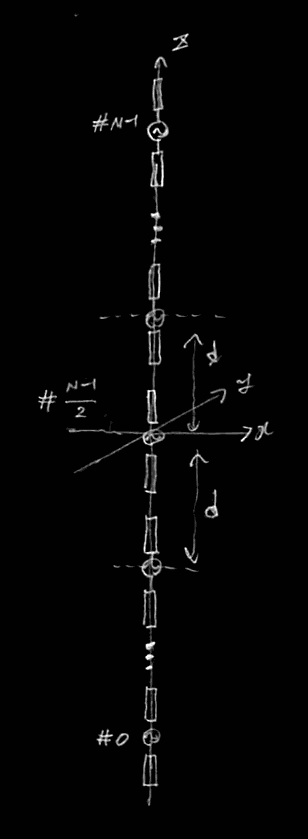
broadside型は完全半波長ダイポールアンテナを素子間隔$d$を隔てて素子と並行な直線上に配列したものである。次の図はz軸方向に$N$本の素子を配列した様子である( 絵が下手なのはご愛嬌 )。
 broadsideアレイアンテナの配列図
上図は$N$が奇数の場合である。偶数の場合は原点を挟んで上下にそれぞれ$d/2$だけずれた位置に素子が置かれることになる。最も下にある素子を#0と番号付けし、上に行くにつれて番号を1つずつ増やしていく。
全ての素子の電流の振幅を等しくし、番号が1増えるごとに電流の位相を$\delta$だけ増やした場合の、位相の基準を原点にとった「配列係数」は次式で与えられる(文献[1] 52頁)。導出は後述するend-fire型よりも容易であり、end-fire型の導出は本記事でこの後述べる。
\begin{equation}
f_N(\theta) = \frac{\sin(N\psi/2)}{N\sin(\psi/2)} \label{配列係数}
\end{equation}
ここに$\psi = kd\sin\theta + \delta$、$k=2\pi/\lambda$は波数である。 念のために触れておくと、$\lim_{\psi\to 0}f_N(\theta) = 1$である。 これと素子自体が持つ指向性の積がアンテナ系全体の指向性$D_\mathrm{t}(\theta,\varphi)$となり(文献[1] 52頁)、\eqref{完全半波長ダイポールアンテナの遠方領域での放射電界}より $D_\mathrm{t}(\theta,\varphi)$ は次式となる。
\[ D_\mathrm{t}(\theta,\varphi) = D(\theta)\frac{\sin(N\psi/2)}{N\sin(\psi/2)} \quad \text{where} \quad D(\theta) := \frac{\cos\left(\frac{\pi}{2}\cos\theta\right)}{\sin\theta} \]
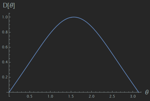
下図は$D(\theta)$をプロットしたものである。
 アンテナ素子の指向性関数のプロット
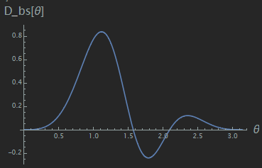
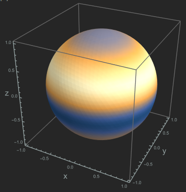
このことから、z軸方向の放射強度は必ず0になる。よってbroadside型は上下に指向性を向けられるが、強放射領域はドーム型ではなく$z$軸を取り巻くリング状になる。下の図は$d=0.4\lambda$、$f_N(\theta)$の最大放射方向$=\pi/3$としたときの放射強度分布をプロットしたものである。強度が負の場所はフェーザの位相が反転することを意味する。
 broadside型アレイアンテナの放射強度分布のプロット
 broadside型アレイアンテナの放射強度分布の球面プロット
end-fire型
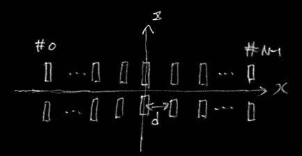
下図のように、完全半波長ダイポールアンテナを$x$軸方向に$N$本配列する。
 x軸上に配列されたダイポールアンテナ
アレイの中心の電流位相を基準とし、$x$座標が最も小さいものを#0、最も大きいものを#N-1と番号付けする。原点から十分離れた位置$\bm{r}$に於ける放射電界のフェーザは、アレイを構成する各素子からの放射電界のフェーザすなわち式\eqref{完全半波長ダイポールアンテナの遠方領域での放射電界}を加算して求める。
そのためにまず、原点から$x$軸の正の向きに$d$だけ離れた位置に置かれた素子による放射電界のフェーザを求めておく。素子に対する観測点の相対座標を$\tilde{\bm{r}}$、その大きさを$\tilde{r}$とする。$\tilde{\bm{r}}$と$z$軸の正の向きが成す角を$\tilde{\theta}$とする。
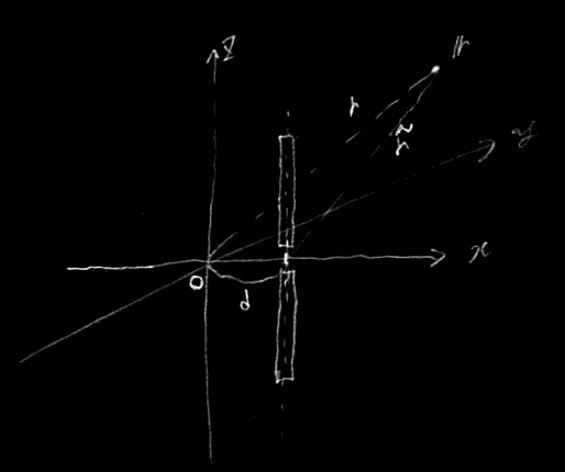 x=dの位置に置かれたダイポールアンテナ
式\eqref{完全半波長ダイポールアンテナの遠方領域での放射電界}この素子による放射電界は次式である。
$$
\begin{aligned}
\bm{E}(d,r,\theta,\varphi) &= j60I_0\frac{e^{-jk\tilde{r}}}{\tilde{r}}\frac{\cos\left(\frac{\pi}{2}\cos\tilde{\theta}\right)}{\sin\tilde{\theta}}\bm{i}_{\tilde{\theta}} \\
&\approx j60I_0\frac{e^{-jk\tilde{r}}}{r}\frac{\cos\left(\frac{\pi}{2}\cos\theta\right)}{\sin\theta}\bm{i}_\theta \\
&\approx j60I_0\frac{e^{-jkr+jkd\sin\theta\cos\varphi}}{r}\frac{\cos\left(\frac{\pi}{2}\cos\theta\right)}{\sin\theta}\bm{i}_\theta
\end{aligned}
$$
上から2つ目の式の導出には次の事実を用いた。
$$
\begin{aligned}
\tilde{r} &\approx r – \frac{\bm{r}}{r}\cdot[d,0,0]^\top = r – [\sin\theta\cos\varphi,\sin\theta\sin\varphi,\cos\theta][d,0,0]^\top \\
&= r – d\sin\theta\cos\varphi
\end{aligned}
$$
この関係式の導出は別の記事で述べている。
これを用いてアレイの放射電界を求める。素子番号の増加とともに電流の位相を$\delta$だけ増加させるものとする。$N$本の素子の合成電界のフェーザ$\bm{E}_\mathrm{EF}(r,\theta,\varphi)$は次式である。
$$
\begin{aligned}
\bm{E}_\mathrm{EF}(r,\theta,\varphi) &= \sum_{n=0}^{N-1} e^{j\delta(n-(N-1)/2)}\bm{E}\left(d\bigl(n-(N-1)/2\bigr),r,\theta,\varphi\right) \\
&\approx j60I_0\frac{e^{-jkr}}{r}\frac{\cos\left(\frac{\pi}{2}\cos\theta\right)}{\sin\theta}\bm{i}_\theta \sum_{n=0}^{N-1} e^{j\psi(n-(N-1)/2)} \quad (\psi = \delta + kd\sin\theta\cos\varphi) \\
&= j60I_0\frac{e^{-jkr}}{r}\frac{\cos\left(\frac{\pi}{2}\cos\theta\right)}{\sin\theta}\frac{\sin(N\psi/2)}{\sin(\psi/2)}\bm{i}_\theta
\end{aligned}
$$
$\sin(N\psi/2)/\sin(\psi/2)$は$2\pi$周期関数であり、$\sin\theta\cos\varphi=-\delta/(kd)+2m\pi\;(m\in\integers)$となるような$\theta,\varphi$に対して最大となる。最大値が1となるように規格化したものが前述の式\eqref{配列係数}である。$x$軸に平行な平面上では$\sin\theta\cos\varphi$が一定であるため、この配列係数は$x$軸周りに対称な形状をしている。
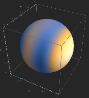
下の図は$d=0.4\lambda$、最大放射方向を$\theta=\pi/2,\varphi=0$としたときの放射強度分布をプロットしたものである。
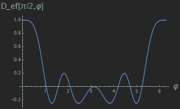 end-fire型アレイアンテナの放射強度分布
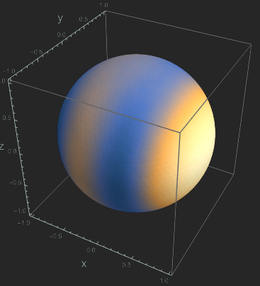 end-fire型アレイアンテナの放射強度分布の球面プロット
broadside型と異なり、最大放射方向の中心に穴が無い。
可視化用Mathematicaコード
前掲の強度分布の計算に使ったMathematicaコードを示す。
コメントを残す
コメントを投稿するにはログインしてください。