はじめに
とあるクロック・バッファのデータ・シートを見ていると、差動入力のコモン電圧をバイアスする使い方の回路図が示されていた。自分はエレキを生業としていないが、ふと気になって入力インピーダンスが終端抵抗とほぼ等しくなることを確かめたくなった。本記事ではその計算過程を示す。
\[
% to cope with definition mismatch between MathJax and LaTeX
\newcommand{\coloneq}{\mathrel{:=}}
\newcommand{\eqcolon}{\mathrel{=:}}
% general purpose
\newcommand{\ctext}[1]{\raise0.2ex\hbox{\textcircled{\scriptsize{#1}}}}
% mathematics
% general purpose
\DeclarePairedDelimiterX{\parens}[1]{\lparen}{\rparen}{#1}
\DeclarePairedDelimiterX{\braces}[1]{\lbrace}{\rbrace}{#1}
\DeclarePairedDelimiterX{\bracks}[1]{\lbrack}{\rbrack}{#1}
\DeclarePairedDelimiterX{\verts}[1]{|}{|}{#1}
\DeclarePairedDelimiterX{\Verts}[1]{\|}{\|}{#1}
\DeclarePairedDelimiterX{\setComprehension}[2]{\lbrace}{\rbrace}{#1\,\delimsize\vert\,#2}
\newcommand{\as}{{\quad\textrm{as}\quad}}
\newcommand{\st}{{\textrm{ s.t. }}}
\newcommand{\naturalNumbers}{\mathbb{N}}
\newcommand{\integers}{\mathbb{Z}}
\newcommand{\rationalNumbers}{\mathbb{Q}}
\newcommand{\realNumbers}{\mathbb{R}}
\newcommand{\nonNegRealNumbers}{\mathbb{R}_{\geq 0}}
\newcommand{\posRealNumbers}{\mathbb{R}_{> 0}}
\newcommand{\complexNumbers}{\mathbb{C}}
\newcommand{\field}{\mathbb{F}}
\newcommand{\EuclideanSpace}{\mathbb{E}}
\newcommand{\argmax}{\operatorname*{arg~max}}
\newcommand{\argmin}{\operatorname*{arg~min}}
% set theory
\newcommand{\range}[2]{\braces*{#1,\dotsc,#2}}
\renewcommand{\complement}{\mathrm{c}}
\newcommand{\ind}[2]{\mathbbm{1}_{#1}\parens*{#2}}
\newcommand{\indII}[1]{\mathbbm{1}\braces*{#1}}
% number theory
\newcommand{\abs}[1]{\verts*{#1}}
\newcommand{\combi}[2]{{_{#1}\mathrm{C}_{#2}}}
\newcommand{\perm}[2]{{_{#1}\mathrm{P}_{#2}}}
\newcommand{\GaloisField}{\mathrm{GF}}
% real analysis
\newcommand{\NapierE}{\mathrm{e}}
\newcommand{\sgn}{\operatorname{sgn}} % sign function
\newcommand{\rect}{\operatorname{rect}} % rectangular function
\newcommand{\cl}{\operatorname{cl}} % closure of a set
\newcommand{\img}{\operatorname{im}} % image of a function
\newcommand{\dom}{\operatorname{dom}} % domain of a function
\newcommand{\LittleO}[2]{\underset{#1}{o}\parens*{#2}} % little-o notation
\newcommand{\norm}[1]{\Verts*{#1}} % norm of a vector or function
\newcommand{\floor}[1]{\left\lfloor #1\right\rfloor}
\newcommand{\ceil}[1]{\left\lceil#1\right\rceil}
\newcommand{\sinc}{\operatorname{sinc}}
\newcommand{\nrmSinc}{\operatorname{nsinc}} % normalized sinc function
\newcommand{\erf}{\operatorname{erf}}
% inverse trigonometric functions
\newcommand{\asin}{\operatorname{Sin}^{-1}}
\newcommand{\acos}{\operatorname{Cos}^{-1}}
\newcommand{\atan}{\operatorname{Tan}^{-1}}
% derivative
\newcommand{\deriv}[3]{\frac{\mathrm{d}^{#3}#1}{\mathrm{d}{#2}^{#3}}}
\newcommand{\derivLong}[3]{\frac{\mathrm{d}^{#3}}{\mathrm{d}{#2}^{#3}}#1}
\newcommand{\partDeriv}[3]{\frac{\mathrm{\partial}^{#3}#1}{\mathrm{\partial}{#2}^{#3}}}
\newcommand{\partDerivLong}[3]{\frac{\mathrm{\partial}^{#3}}{\mathrm{\partial}{#2}^{#3}}#1}
\newcommand{\partDerivIIHetero}[3]{\frac{\mathrm{\partial}^2#1}{\partial#2\mathrm{\partial}#3}}
\newcommand{\partDerivIIHeteroLong}[3]{{\frac{\mathrm{\partial}^2}{\partial#2\mathrm{\partial}#3}#1}}
% integral
\newcommand{\pv}{{\textrm{ p.v. }}}
\newcommand{\integrate}[5]{\int_{#1}^{#2}{#3}{\;\mathrm{d}^{#4}}#5}
\newcommand{\LebInteg}[4]{\int_{#1} {#2} {#3}\parens*{\;\mathrm{d}#4}}
% complex analysis
\newcommand{\conj}[1]{\overline{#1}}
\renewcommand{\Re}{\operatorname{Re}}
\renewcommand{\Im}{\operatorname{Im}}
\newcommand{\Arg}{\operatorname{Arg}}
\newcommand{\Log}{\operatorname{Log}}
% Laplace transform
\newcommand{\LPLC}{\operatorname{\mathcal{L}}}
\newcommand{\ILPLC}{\operatorname{\mathcal{L}}^{-1}}
% discrete fourier transform
\newcommand{\DFT}{\operatorname{DFT}}
\newcommand{\IDFT}{\operatorname{IDFT}}
% Z-transform
\newcommand{\ZTrans}{\operatorname{\mathcal{Z}}}
\newcommand{\IZTrans}{\operatorname{\mathcal{Z}}^{-1}}
\newcommand{\SSZTrans}{\underset{\text{s.s.}}{\mathcal{Z}}} % single-sided Z-transform
% linear algebra
\newcommand{\bm}[1]{{\boldsymbol{#1}}}
\newcommand{\vecEntry}[2]{\bm{#1}\bracks*{#2}}
\newcommand{\matEntry}[3]{#1\bracks*{#2}\bracks*{#3}}
\newcommand{\matPart}[5]{\matEntry{#1}{#2:#3}{#4:#5}}
\newcommand{\minor}[3]{{#1}\bracks*{\setminus #2}\bracks*{\setminus #3}} % the minor of a matrix: row #2 and column #3 deleted
\newcommand{\diag}{\operatorname{diag}}
\newcommand{\transpose}[1]{{#1}^\top}
\newcommand{\HerConj}[1]{{#1}^*}
\newcommand{\tr}{\operatorname{tr}}
\newcommand{\inProd}[2]{\left\langle#1,#2\right\rangle}
\newcommand{\dotProd}[2]{#1 \cdot #2}
\newcommand{\HadamardProd}{\odot}
\newcommand{\HadamardDiv}{\oslash}
\newcommand{\vecSpan}{\operatorname{span}}
\newcommand{\rank}{\operatorname{rank}}
% vector
% unit vector
\newcommand{\vix}{\bm{i}_x}
\newcommand{\viy}{\bm{i}_y}
\newcommand{\viz}{\bm{i}_z}
% graph theory
\newcommand{\neighborhood}{\mathcal{N}}
% probability theory
\newcommand{\PDF}{\operatorname{PDF}}
\newcommand{\Ber}{\operatorname{Ber}}
\newcommand{\Beta}{\operatorname{Beta}}
\newcommand{\ExpDist}{\operatorname{ExpDist}}
\newcommand{\ErlangDist}{\operatorname{ErlangDist}}
\newcommand{\PoissonDist}{\operatorname{PoissonDist}}
\newcommand{\GammaDist}{\operatorname{Gamma}}
\newcommand{\cind}[2]{\ind{#1\left| #2\right.}} % conditional indicator function
\renewcommand{\Pr}{\operatorname{Pr}}
\DeclarePairedDelimiterX{\cPrParens}[2]{(}{)}{#1\,\delimsize\vert\,#2}
\newcommand{\Ev}{\operatorname{E}} % expected value
\newcommand{\Var}{\operatorname{Var}}
\newcommand{\Cov}{\operatorname{Cov}}
% physics
% unit of measurement
\newcommand{\second}{\text{s}}
\newcommand{\hertz}{\text{Hz}}
\newcommand{\decibel}{\text{dB}}
% signal processing
% Discrete Time Fourier Transform
\newcommand{\DTFT}{\operatorname{DTFT}}
\newcommand{\IDTFT}{\operatorname{IDTFT}}
% computer science
% fixed-point arithmetic
\newcommand{\IntPartBW}[1]{\underbracket[0.140ex]{#1}_\mathrm{i}} % 0.140ex is half of the default thickness. See: [How to make underbracket thinner](https://tex.stackexchange.com/questions/559078/how-to-make-underbracket-thinner)
\newcommand{\DecPartBW}[1]{\underbracket[0.140ex]{#1}_\mathrm{d}}
\newcommand{\TotalBW}[1]{\underbracket[0.140ex]{#1}}
\newcommand{\Rat}{\operatorname{Rat}} % Maps a fixed-point number to a corresponding rational number.
% programming
\newcommand{\plpl}{\mathrel{++}}
\newcommand{\pleq}{\mathrel{+}=}
\newcommand{\asteq}{\mathrel{*}=}
\]
対象とする回路
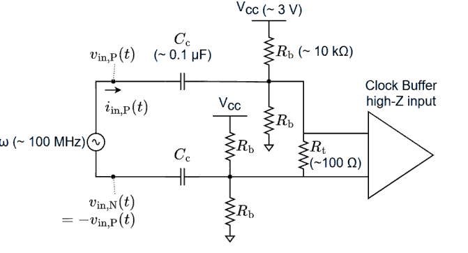 対象とする回路
対象とする回路は、コモン電圧 = 0 V の差動入力の コモン電圧を $V_\text{cc}/2$ に変換してクロック・バッファに入力する回路である。$R_\text{b}$ はバイアス抵抗の抵抗値、$R_\text{t}$ は終端抵抗の抵抗値、$C_\text{c}$ はカップリング・キャパシタの容量である。この回路の入力インピーダンス $Z_\text{in}$ を知りたい。
導出
前掲の図の回路は直流成分と正弦波成分の定常状態にあるものとする(つまり初期値応答は減衰して消えているものとする)。抵抗とキャパシタの端子の電圧を直流成分と正弦波成分に分解して重ね合わせの定理を適用する。カップリング・キャパシタにより電流 $i_\text{in,P}(t)$ の直流成分は 0 であることに注意する。正弦波成分のみに着目すると次の等価回路を得る。
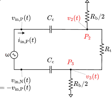 正弦波成分のみに着目した等価回路
この図中の電圧と電流の phasor を使う。小文字で示された時間領域の物理量の phasor を大文字で示す。
接点 $P_2$ と $P_3$ に於いて接点方程式を解くと $V_3 = -V_2$ が容易に解る。これを接点 $P_2$ に於ける接点方程式に適用すると次式を得る。次の図を得る。
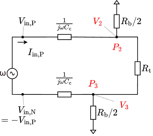 正弦波成分のみに着目した phasor 等価回路
\[
\begin{gather*}
j\omega C_\text{c}(V_2 – V_\text{in,P}) + 2\parens{\frac{1}{R_\text{b}} + \frac{1}{R_\text{t}}}V_2 = 0 \\
\therefore V_2 = \frac{j\omega C_\text{c}}{j\omega C_\text{c} + 2\parens{\frac{1}{R_\text{b}} + \frac{1}{R_\text{t}}}}V_\text{in,P} \\
\therefore I_\text{in,P} = j\omega C_\text{c}(V_\text{in,P} – V_2) = j\omega C_\text{c}\frac{2\parens{\frac{1}{R_\text{b}} + \frac{1}{R_\text{t}}}}{j\omega C_\text{c} + 2\parens{\frac{1}{R_\text{b}} + \frac{1}{R_\text{t}}}}V_\text{in,P} \\
Z_\text{in} = \frac{V_\text{in,P} – (-V_\text{in,P})}{I_\text{in,P}} = 2\frac{j\omega C_\text{c} + 2\parens{\frac{1}{R_\text{b}} + \frac{1}{R_\text{t}}}}{2j\omega C_\text{c}\parens{\frac{1}{R_\text{b}} + \frac{1}{R_\text{t}}}}
\end{gather*}
\]
最初に掲げた図中の抵抗値とキャパシタンスを考慮すると $1/R_\text{b} + 1/R_\text{t}\approx 1/R_\text{t}$、$j\omega C_\text{c} + 2(1/R_\text{b} + 1/R_\text{t})\approx j\omega C_\text{c}$ であるから $Z_\text{in} \approx R_\text{t}$ である(近似せずに計算すると $99.0099 – 0.031831j$ Ω である)。

コメントを残す
コメントを投稿するにはログインしてください。