はじめに
4年近く前に数値解析の講義で3次spline補間を教わったが、最近ふと、これを拡張して2次元の閉曲線を描けないか?と思って考えていた。導出とサンプルプログラムが完成したのでここに書いておく。
定義
$n\in\naturalNumbers$, $t_0 < t_1 < \dotsb < t_n$, $x_i\in\realNumbers\;(i=0,1,\dotsc,n)$とする。区間$I_i \coloneqq [t_i, t_{i+1})\;(i=0,1,\dotsc,n-2),\;I_{n-1} \coloneqq [t_{n-1},t_n]$に対して3次以下の多項式$P_i(t) \coloneqq a_i + b_i(t-t_i) + c_i(t-t_i)^2 + d_i(t-t_i)^3$を定義し、区分的に定義された多項式関数
\[ S(t) \coloneqq \sum_{i=0}^{n-1} \mathbb{1}_{I_i}(t)P_i(t) \]
を定義する($\mathbb{1}_A(t)$は集合$A$の指示関数である)。$P_i$には次の制約を課す。
- $P_i(t_i) = x_i\;(i=0,1,\dotsc,n-1)$
- $P_{n-1}(t_n) = x_n$
- $P_i(t_i) = P_{i-1}(t_i)\;(i=1,\dotsc,n-1)$
- ${P_i}'(t_i) = {P_{i-1}}'(t_i)\;(i=1,\dotsc,n-1)$
- ${P_i}”(t_i) = {P_{i-1}}”(t_i)\;(i=1,\dotsc,n-1)$
- ${P_0}”(t_0) = {P_{n-1}}”(t_n) = 0$
条件1,2は曲線$S(t)$が「ノット」$(t_i,x_i)$を通ることを意味する。条件3,4,5は隣接する区間の境界で曲線の2階の微分係数までが一致する(つまり滑らかに繋がっている)ことを意味する。条件6は人工的だが、曲線が両端の近くで直線になることを意味する。この条件により、上述の$S(t)$の定義域はノットの外側まで拡張できて、
\[ S(t) \coloneqq \begin{cases} P_0(t_0) + {P_0}'(t_0)(t-t_0) = a_0 + b_0(t-t_0) & (t < t_0) \\ \sum_{i=0}^{n-1} \mathbb{1}_{I_i}(t)P_i(t) & (t_0 \leq t \leq t_n) \\ P_{n-1}(t_n) + {P_{n-1}}'(t_n)(t-t_n) & (t > t_n) \end{cases} \]
となる。パラメータは$a_i,b_i,c_i,d_i\;(i=0,1,\dotsc,n-1)$の$4n$個、制約条件も$4n$個だからパラメータが一意に決まると期待できる。
$P_i(t)$の計算
条件1より$a_i = x_i\;(i=0,1,\dotsc,n-1)$が確定する。 $b_i$を$c_i,d_i$で表して$c_i,d_i$を求めてから$b_i$を求める方針で考える。条件3より
\begin{align*} b_{i-1} &= \frac{1}{t_i-t_{i-1}}\left[a_i-a_{i-1} – c_{i-1}(t_i-t_{i-1})^2 – d_{i-1}(t_i-t_{i-1})^3\right] \\ &= \frac{a_i-a_{i-1}}{t_i-t_{i-1}} – c_{i-1}(t_i-t_{i-1}) – d_{i-1}(t_i-t_{i-1})^2 \; (i=1,\dotsc,n-1) \end{align*}
条件2に注意すると、$a_n \coloneqq x_n$とすることで上式は$i=n$のときも成り立つので、次式を得る。
\begin{equation} b_i = \frac{a_{i+1}-a_i}{t_{i+1}-t_i} – c_i(t_{i+1}-t_i) – d_i(t_{i+1}-t_i)^2 \; (i=0,\dotsc,n-1) \label{biをai,ci,di表した式} \end{equation}
条件4より
\[ b_i = b_{i-1} + 2c_{i-1}(t_i-t_{i-1}) + 3d_{i-1}(t_i-t_{i-1})^2 \; (i=1,\dotsc,n-1)\]
この式に\eqref{biをai,ci,di表した式}を適用して
\begin{align} &\phantom{=} \frac{a_{i+1}-a_i}{t_{i+1}-t_i} – c_i(t_{i+1}-t_i) – d_i(t_{i+1}-t_i)^2 = \frac{a_i-a_{i-1}}{t_i-t_{i-1}} – c_{i-1}(t_i-t_{i-1}) – d_{i-1}(t_i-t_{i-1})^2 \nonumber \\ &\phantom{=} + 2c_{i-1}(t_i-t_{i-1}) + 3d_{i-1}(t_i-t_{i-1})^2 \nonumber \\ \therefore\; &\phantom{=} – c_i(t_{i+1}-t_i) – d_i(t_{i+1} – t_i)^2 = \frac{a_i-a_{i-1}}{t_i-t_{i-1}} – \frac{a_{i+1}-a_i}{t_{i+1}-t_i} + c_{i-1}(t_i-t_{i-1}) + 2d_{i-1}(t_i – t_{i-1})^2 \nonumber \\ \therefore\; &\phantom{=} d_i(t_{i+1}-t_i)^2 = \frac{a_{i+1}-a_i}{t_{i+1}-t_i} – \frac{a_i-a_{i-1}}{t_i-t_{i-1}} – c_i(t_{i+1}-t_i) – c_{i-1}(t_i-t_{i-1}) – 2d_{i-1}(t_i-t_{i-1})^2 \label{diをci,cim1,dim1で表した式} \end{align}
条件5より
\begin{equation} c_i = c_{i-1} + 3d_{i-1}(t_i-t_{i-1}) \; (i=1,\dotsc,n-1) \label{ciをcim1,dim1で表した式} \end{equation}
この式を\eqref{diをci,cim1,dim1で表した式}に適用して整理すると次式を得る。
\begin{equation} d_i = \frac{1}{(t_{i+1}-t_i)^2}\left[\frac{a_{i+1}-a_i}{t_{i+1}-t_i} – \frac{a_i-a_{i-1}}{t_i-t_{i-1}} – c_{i-1}(t_{i+1}-t_{i-1}) – d_{i-1}(t_i-t_{i-1})(3t_{i+1}-t_i-2t_{i-1})\right] \label{diをcim1,dim1で表した式} \end{equation}
\eqref{ciをcim1,dim1で表した式},\eqref{diをcim1,dim1で表した式}より$c_i,d_i\;(i=1,\dotsc,n-1)$が$c_0,d_0$の一次式で表されることが解るが、条件6より$c_0 = 0$なので$d_0$の一次式となる。また、再び条件6より次式が成り立つ。
\begin{equation} c_{n-1} + 3d_{n-1}(t_n-t_{n-1}) = 0 \label{cnm1とdnm1の関係式} \end{equation}
以上より、\eqref{ciをcim1,dim1で表した式},\eqref{diをcim1,dim1で表した式}を用いて$c_i,d_i$を$d_0$の一次式で表してから\eqref{cnm1とdnm1の関係式}で$d_0$を求めれば$c_i,d_i$が求まり、\eqref{biをai,ci,di表した式}で$b_i$が求まる。具体的には、$c_i = \alpha_i + \beta_i d_0,\; d_i = \gamma_i + \delta_i d_0$と表すことを考え、次の漸化式を計算する。
\[ \alpha_0 = \beta_0 = 0,\;\gamma_0 = 0,\;\delta_0 = 1 \]
\begin{align*} &\text{for } i=1,2,\dotsc,n-1 \text{:} \\ \alpha_i &= \alpha_{i-1} + 3\gamma_{i-1}(t_i-t_{i-1}) \\ \beta_i &= \beta_{i-1} + 3\delta_{i-1}(t_i-t_{i-1}) \\ \gamma_i &= \frac{1}{(t_{i+1}-t_i)^2}\left[\frac{a_{i+1}-a_i}{t_{i+1}-t_i} – \frac{a_i-a_{i-1}}{t_i-t_{i-1}} – \alpha_{i-1}(t_{i+1}-t_{i-1}) – \gamma_{i-1}(t_i-t_{i-1})(3t_{i+1} – t_i – 2t_{i-1}) \right] \\ \delta_i &= \frac{1}{(t_{i+1}-t_i)^2}\left[-\beta_{i-1}(t_{i+1}-t_{i-1}) – \delta_{i-1}(t_i-t_{i-1})(3t_{i+1} – t_i – 2t_{i-1})\right] \end{align*}
その後、\eqref{cnm1とdnm1の関係式}から次式を得る。
\[ \alpha_{n-1} + 3\gamma_{n-1}(t_n-t_{n-1}) + d_0[\beta_{n-1} + 3\delta_{n-1}(t_n-t_{n-1})] = 0 \]
\[ \therefore\; d_0 = -\frac{\alpha_{n-1} + 3\gamma_{n-1}(t_n-t_{n-1})}{\beta_{n-1} + 3\delta_{n-1}(t_n-t_{n-1})} \]
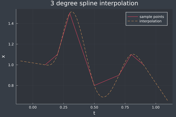
これと$\alpha_i,\beta_i,\gamma_i,\delta_i$を用いて$c_i,d_i$を求めればよい。これを実装したJuliaプログラムコードをここに置いてある(Gistではレンダリングに失敗するので直接DLして実行するのがよい。ipynbが2つ以上あると失敗するように見える)。次の図は、このプログラムで計算したspline曲線である。
2次元以上の曲線への拡張
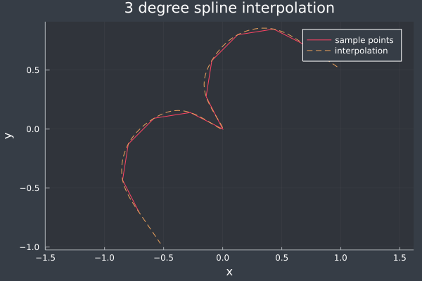
2次元以上の曲線は$t$を媒介変数として表現する。各成分を3次spline関数で表せばよい。次の図は、先程のプログラムで計算した2次元のspline曲線である。
巡回的な境界条件
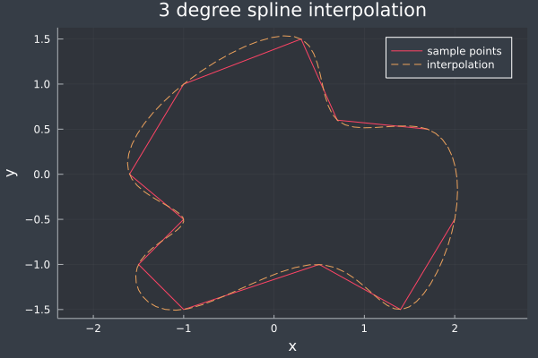
次のような巡回的な境界条件を考えることができる。これは2次元以上の閉曲線を考える際に必須である。
- $P_i(t_i) = P_{i-1}(t_i)\;(i=1,2,\dotsc,n-1)$
- $P_0(t_0) = P_{n-1}(t_n)$
- ${P_i}'(t_i) = {P_{i-1}}'(t_i)\;(i=1,2,\dotsc,n-1)$
- ${P_0}'(t_0) = {P_{n-1}}'(t_n)$
- ${P_i}”(t_i) = {P_{i-1}}”(t_i)\;(i=1,2,\dotsc,n-1)$
- ${P_0}”(t_0) = {P_{n-1}}”(t_n)$
直観的に言えば、1次元の場合であれば、例えば$[-\pi,\pi)$で定義されたspline関数が全区間に滑らかに周期的に拡張できることになる。2次元以上の場合であれば曲線の始点($t=t_0$に対応)が終点($t=t_n$に対応)と滑らかに繋がっている。
条件1,2より$a_i = x_i\;(i=0,1,\dotsc,n-1)$が確定し、さらに次の2つの式が得られる。
\begin{equation} \label{aiをaim1,bim1,cim1,dim1で表した式} a_i = a_{i-1} + b_{i-1}(t_i-t_{i-1}) + c_{i-1}(t_i-t_{i-1})^2 + d_{i-1}(t_i-t_{i-1})^3\;(i=1,2,\dotsc,n-1) \end{equation} \begin{equation} \label{a0をanm1,bnm1,cnm1,dnm1で表した式} a_0 = a_{n-1} + b_{n-1}(t_n-t_{n-1}) + c_{n-1}(t_n-t_{n-1})^2 + d_{n-1}(t_n-t_{n-1})^3 \end{equation}
条件3より
\begin{equation} \label{biをbim1,cim1,dim1で表した式} b_i = b_{i-1} + 2c_{i-1}(t_i-t_{i-1}) + 3d_{i-1}(t_i-t_{i-1})^2\;(i=1,2,\dotsc,n-1) \end{equation}
条件4より
\begin{equation} \label{b0をbnm1,cnm1,dnm1で表した式} b_0 = b_{n-1} + 2c_{n-1}(t_n-t_{n-1}) + 3d_{n-1}(t_n-t_{n-1})^2 \end{equation}
条件5より
\begin{equation} \label{巡回的な境界条件の場合_ciをcim1,dim1で表した式} c_i = c_{i-1} + 3d_{i-1}(t_i-t_{i-1}) \end{equation}
条件6より
\begin{equation} \label{c0をcnm1,dnm1で表した式} c_0 = c_{n-1} + 3d_{n-1}(t_n-t_{n-1}) \end{equation}
直ぐに思いつくのは「$P_i(t)$の計算」と同様に$c_{n-1},d_{n-1}$を$c_0,d_0$で表して、境界条件から$c_0,d_0$を決定する方針であるが、これでは上手くいかない。\eqref{a0をanm1,bnm1,cnm1,dnm1で表した式},\eqref{b0をbnm1,cnm1,dnm1で表した式}より、$b_0$と$c_{n-1},d_{n-1}$が相互依存しているためである。今回は$b_{n-1}$も漸化式に組み込む必要がある。ここまでに登場した式を見れば$b_i,c_i,d_i$が$b_{i-1},c_{i-1},d_{i-1}$の一次式となるので$b_{n-1},c_{n-1},d_{n-1}$も当然そうなる。そこで、適当な$3\times 3$行列$A_i,B_i$と3次列ベクトル$\bm{k}_i,\bm{l}_i$を用いて
\begin{equation} \label{bi,ci,diをb0,c0,d0で表した式} [b_i,c_i,d_i]^\top = B_i[b_{i-1},c_{i-1},d_{i-1}]^\top + \bm{l}_i, \quad [b_i,c_i,d_i]^\top = A_i[b_0,c_0,d_0]^\top + \bm{k}_i \end{equation}
\[ A_0 \coloneqq I,\; \bm{k}_0 \coloneqq \bm{0},\; A_i = B_i A_{i-1},\;\bm{k}_i = B_i\bm{k}_{i-1} + \bm{l}_i \]
と表すことを考える。$B_i$の1,2行目は\eqref{biをbim1,cim1,dim1で表した式},\eqref{巡回的な境界条件の場合_ciをcim1,dim1で表した式}から容易に解る。\eqref{aiをaim1,bim1,cim1,dim1で表した式}より
\begin{equation} \label{diをaip1,ai,bi,ciで表した式} d_i = \frac{a_{i+1}-a_i}{(t_{i+1}-t_i)^3} – \frac{b_i}{(t_{i+1}-t_i)^2} – \frac{c_i}{(t_{i+1}-t_i)}\;(i=0,1,\dotsc,n-2) \end{equation}
\eqref{a0をanm1,bnm1,cnm1,dnm1で表した式}より、$a_n \coloneqq a_0$とすることで上の式は$i=n-1$まで拡張できる。これに\eqref{biをbim1,cim1,dim1で表した式},\eqref{巡回的な境界条件の場合_ciをcim1,dim1で表した式}を適用して整理すると次式を得る。
\begin{equation} \label{diをaip1,ai,bim1,cim1,dim1で表した式} d_i = \frac{a_{i+1}-a_i}{{h_{i+1}}^3} – \frac{b_{i-1}}{{h_{i+1}}^2} – \frac{c_{i-1}}{{h_{i+1}}^2}(2h_i + h_{i+1}) – \frac{3d_{i-1}}{{h_{i+1}}^2}h_i(h_i + h_{i+1}) \; (h_i \coloneqq t_i-t_{i-1}) \end{equation}
以上より$B_i,\bm{l}_i$は次のようになる。
\[ B_i = \begin{bmatrix} 1 & 2h_i & 3{h_i}^2 \\ 0 & 1 & 3h_i \\ -\frac{1}{{h_{i+1}}^2} & -\frac{2h_i + h_{i+1}}{{h_{i+1}}^2} & -\frac{3}{{h_{i+1}}^3}h_i(h_i + h_{i+1}) \end{bmatrix},\quad \bm{l}_i = \left[0, 0, \frac{a_{i+1}-a_i}{{h_{i+1}}^3}\right]^\top \]
$b_{i-1},c_{i-1},d_{i-1}$の満たすべき条件を考える。\eqref{a0をanm1,bnm1,cnm1,dnm1で表した式}は\eqref{diをaip1,ai,bim1,cim1,dim1で表した式}を導くのに既に使っているから新たな情報にはならない。\eqref{b0をbnm1,cnm1,dnm1で表した式},\eqref{c0をcnm1,dnm1で表した式}より次式が成り立つ。
\[ \begin{bmatrix} 1 & 2h_n & 3{h_n}^2 \\ 0 & 1 & 3h_n \end{bmatrix} [b_{n-1}, c_{n-1}, d_{n-1}]^\top = [b_0, c_0]^\top \]
左辺の行列を$M_1$とおいて式変形を進めると
\begin{align*} &\phantom{\iff} M_1\left(A_{n-1}[b_0, c_0, d_0]^\top + \bm{k}_{n-1}\right) = [b_0, c_0]^\top \\ &\iff (M_1A_{n-1} – M_2)[b_0, c_0, d_0]^\top = -M_1\bm{k}_{n-1} \quad \left(M_2 \coloneqq \begin{bmatrix} 1 & 0 & 0 \\ 0 & 1 & 0 \end{bmatrix} \right) \end{align*}
$b_0,c_0,d_0$を決定するにはもう一つ条件式が必要である。\eqref{diをaip1,ai,bi,ciで表した式}で$i=0$とおくと次式を得る。
\[ h_1b_0 + {h_1}^2 c_0 + {h_1}^3d_0 = a_1-a_0 \]
以上より、次の方程式を解いて$b_0,c_0,d_0$を求めればよい。
\[ \begin{bmatrix} \quad & M_1A_{n-1} – M_2 & \quad \\ h_1 & {h_1}^2 & {h_1}^3 \end{bmatrix} \begin{bmatrix} b_0 \\ c_0 \\ d_0 \end{bmatrix} = \begin{bmatrix} -M_1\bm{k}_{n-1} \\ a_1 – a_0 \end{bmatrix} \]
その後\eqref{bi,ci,diをb0,c0,d0で表した式}を用いて$b_i,c_i,d_i$を求めればよい。これを実装したJuliaプログラムコードをここに置いてある。次の図は、このプログラムで計算した2次元のspline閉曲線である。